The resulting INES model is an energy system planning model that identifies investment needs and pathways to reach climate neutrality by 2050. To run this planning model, you need two core components:
- An optimization tool — in this case, SpineOpt.
- A time-series clustering tool to reduce temporal dimensionality while preserving operability and long-term storage behavior.
This guide explains how to connect SpineOpt to the INES model and how to run the optimization with clustering.
How to Connect SpineOpt
As part of INES, there is a repository of INES tools that handle data transformations (e.g., transforming INES models to SpineOpt, PyPSA, Flextool, etc.). In this guide, we focus on SpineOpt.
Important: SpineOpt is a plugin for Spine Toolbox. Install it following the official instructions:
- SpineOpt installation: https://spine-tools.github.io/SpineOpt.jl/latest/getting_started/installation/
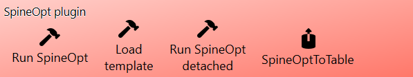
Once installed, Spine Toolbox will include a new item bar with SpineOpt items:
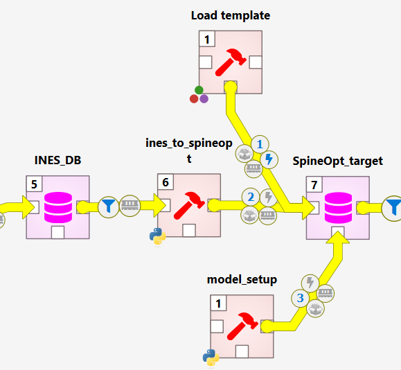
Your goal is to connect SpineOpt to the INES model as illustrated below. The following sections explain each component and how to add them.
Elements
Load template
Spine databases use structural templates that are populated by tools or importers. SpineOpt reads a specific template to build the JuMP optimization model to be solved by a solver. See the concept reference:
- SpineOpt parameters: https://spine-tools.github.io/SpineOpt.jl/latest/concept_reference/Parameters/
In Spine Toolbox:
- From the SpineOpt item bar, drag and drop Load template.
- Set the tool argument to your SpineOpt DB (target database).
ines-spineopt (INES → SpineOpt transformation)
This is a Python-based transformer that converts the INES model into a SpineOpt model.
- Clone the repository and switch to the Pan-European case branch:
git clone https://github.com/ines-tools/ines-spineopt.git
cd ines-spineopt
git checkout EU_case
Note: For the Pan-European framework, use the
EU_casebranch, which is tailored to this case study. A more general transformer will be developed to support any case study. - In Spine Toolbox, create a Python tool to run the transformer:
- Main program:
ines_to_spineopt.py - Tool arguments (in order):
- INES DB (source database)
- SpineOpt DB (target database)
- Tool properties: Set Source directory to the root of the cloned
ines-spineoptrepository.
- Main program:
model setup (final parameterization for optimization)
This is a Python-based tool that manipulates the SpineOpt database to add/modify parameters before optimization.
- Create a Python tool in Spine Toolbox using this script:
- Script: https://github.com/spine-tools/Pan-European-Framework-Energy-System-Planning/blob/main/src/_planning-input-processsing/planning_setup.py
- Tool argument: the SpineOpt DB
- Source directory: set to the root of the Pan-European Framework repository:
- What the script does (economic settings & modeling assumptions):
- Investment cost annualization for investable technologies (decades 2030, 2040, 2050) using WACC.
- If a technology-specific discount rate is not provided, a 5% default is used.
- The optimization horizon ends in 2060. Investments are paid until the end of their lifetime or 2060, whichever comes first.
-
Annuity stream over the lifetime. For an investment made in year y, we first compute the annuity amount A using the technology discount rate r (default 5%) and the number of payment years n = min(lifetime, 2060 − y + 1):
Formula:
A = CAPEX_y * r / (1 - (1 + r)^(-n))The model pays A every year from t = y to t = y + n − 1. Each annual payment is expressed in 2025 currency by deflating with the inflation rate π (default 3%):
Formula:
Payment_2025(t) = A / (1 + π)^(t - 2025)Example: If you invest in 2030 with a 25‑year lifetime, payments occur in 2030…2054, each deflated back to 2025. Do not discount again by r; it is already embedded in the annuity A.
- You can modify inflation, technology discount rate, and the end of the horizon in the script.
- Vintage fixed-cost correction for future technologies: since fixed O&M tends to decrease or remain constant over time, the script ensures that vintage units reflect the fixed cost corresponding to the investment year. By default, the 2050 fixed cost is used, and an additional correction is added to investments realized in 2030 or 2040 based on operational years—this approximates vintage operations.
- Variable cost trajectories are considered to decrease per decade for maturing technologies or remain constant for high-TRL technologies. For instance, a unit invested in 2030 will have a different variable cost in 2040. Note that this is an assumption.
- Heat pump split constraint: 30% of heat pump investments must be ground-source. This avoids the optimizer selecting only the cheapest option while still honoring COP differences. You can change the percentage or disable the constraint.
- Solver settings: the script sets Gurobi as solver by default. You can change this in the model section of the SpineOpt DB using the Spine DB editor.
- Investment cost annualization for investable technologies (decades 2030, 2040, 2050) using WACC.
How to Optimize the SpineOpt Model
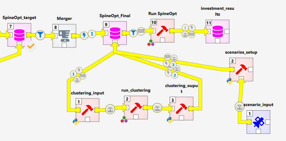
The figure below shows how to connect the SpineOpt DB from the previous section to the optimization workflow:
Elements
merger
Use a Merger to decouple the initial SpineOpt DB from the final one used for optimization. This allows you to keep a clean, reproducible final database for runs.
Final SpineOpt DB
Create an additional SpineOpt DB that will be the final input to the optimization.
SpineOpt Result DB
Add another Spine DB that will store results produced by SpineOpt (e.g., variables and parameters after the run).
Run SpineOpt
From the SpineOpt item bar, drag and drop Run SpineOpt and set the tool arguments:
- Final SpineOpt DB (input)
- SpineOpt Result DB (output)
Clustering (representative periods)
To correctly capture operations across decades, the framework runs one year per decade with a weight of ten, and each year is represented by representative periods. Periods are linked to preserve seasonality and long-term storage behavior by blending representative periods to model the represented ones. See the preprint for more details:
- Preprint: https://arxiv.org/abs/2508.21641
- Tool: TulipaClustering.jl — https://github.com/TulipaEnergy/TulipaClustering.jl
This part consists of three elements:
1) Clustering input
Reads time series from the SpineOpt DB (capacity factors, demand, inflows, nodal flows) and builds the TulipaClustering input. Because of the large number of time series, profiles belonging to the same technology or concept (e.g., wind capacity factors) are averaged to reduce noise. This is an assumption of the framework.
- Create a Python tool with the script:
- Tool argument: the SpineOpt DB
- Tool properties: execute in the source directory (repository root)
- Ensure a subfolder named
_profilesexists; the TulipaClustering input files are exported there.
2) Run clustering
This is a Julia script that runs TulipaClustering.jl using the generated inputs.
- Script: https://github.com/spine-tools/Pan-European-Framework-Energy-System-Planning/blob/main/src/_clustering/tulipa_call.jl
- Configure in the script:
- Representative period length (e.g., 24h for representative days)
- Number of representative periods
- This framework is designed to use representative days to capture solar patterns well.
- Tool properties: execute in the source directory.
- Ensure a subfolder named
_resultsexists inside the clustering folder to store the outputs.
3) Clustering output
This Python script reads the selected representative periods from TulipaClustering and creates representative blocks in the SpineOpt model.
- Script: https://github.com/spine-tools/Pan-European-Framework-Energy-System-Planning/blob/main/src/_clustering/clustering_output.py
- Tool arguments: the Final SpineOpt DB
- Tool properties: execute in the source directory.
scenario input
This is a data connection to the scenario configuration file used by the optimization model. In the Pan-European Framework repository, the file is located under the planning input processing folder:
What you can configure:
scenariosection: define the name of the scenario to run and a list of alternatives included in the scenario (note: clustering adds new alternatives to the model).emission_factorsection: a conversion factor for the emission node and CO₂ storage, defined at European level. If you model one country, set this factor to 30 so the framework divides these values accordingly.resolutionsection: sets the temporal resolution. If using representative periods, 24h is the maximum; otherwise choose any resolution within a one-year horizon.short_term_storage/long_term_storagesections: list which storages are treated as short-term or long-term to correctly link periods when representative periods are used.
scenario setup
This tool imports the scenario configuration into the Final SpineOpt DB.
- Script: https://github.com/spine-tools/Pan-European-Framework-Energy-System-Planning/blob/main/src/_planning-input-processsing/scenario_run.py
- Tool arguments (in order):
- Final SpineOpt DB
- Scenario configuration file (the YAML above)
- Tool properties: execute in the source directory.
Run!
After wiring the workflow:
- Run
ines-spineoptto transform INES → SpineOpt. - Run
model setupto apply economic, solver, and output configurations. - (Optional) Run the clustering chain:
clustering_input→tulipa_call.jl→clustering_output. - Import the scenario:
scenario input→scenario setup. - Run SpineOpt with the Final SpineOpt DB as input and the SpineOpt Result DB as output.
You’re done—inspect results in the results database!
Notes & Tips
- Ensure Julia, Python, and your solver (e.g., Gurobi) are correctly installed and licensed before running.
- Always execute tools in their repository source directories (via tool properties) so relative paths work as expected.
- If you change decade sets, WACC, inflation, or horizon end year, re-run the
model setuptool so the adjustments are reflected in the DB. - When using representative periods, check that storage linking is configured (short/long-term lists) to preserve seasonal dynamics.