Case Study A5 tutorial
Welcome to this Spine Toolbox Case Study tutorial. Case Study A5 is one of the Spine Project case studies designed to verify Toolbox and Model capabilities. To this end, it reproduces an already existing study about hydropower on the Skellefte river, which models one week of operation of the fifteen power stations along the river.
Introduction
Model assumptions
For each power station in the river, the following information is known:
- The capacity, or maximal electricity output. This datum also provides the maximal water discharge as per the efficiency curve (see next point).
- The efficiency curve, or conversion rate from water to electricity. In this study, a piece-wise linear efficiency with two segments is assumed. Moreover, this curve is monotonically decreasing, i.e., the efficiency in the first segment is strictly greater than the efficiency in the second segment.
- The maximal reservoir level (maximal amount of water that can be stored in the reservoir).
- The reservoir level at the beginning of the simulation period and at the end.
- The minimal amount of water that the plant must discharge at every hour. This is usually zero (except for one of the plants).
- The downstream plant, or next plant in the river course.
- The time that it takes for the water to reach the downstream plant. This time can be different depending on whether the water is discharged (goes through the turbine) or spilled.
- The local inflow, or amount of water that naturally enters the reservoir at every hour. In this study, it is assumed constant over the entire simulation period.
- The hourly average water discharge. It is assumed that before the beginning of the simulation, this amount of water has constantly been discharged at every hour.
The system is operated so as to maximize the total profit over the planning week, while respecting capacity constraints, maximal reservoir level constrains, etc. Hourly profit per plant is simply computed as the product of the electricity price and the production.
Modelling choices
The model of the electric system is fairly simple, only two elements are needed:
- A common electricity node.
- A load unit that takes electricity from that node.
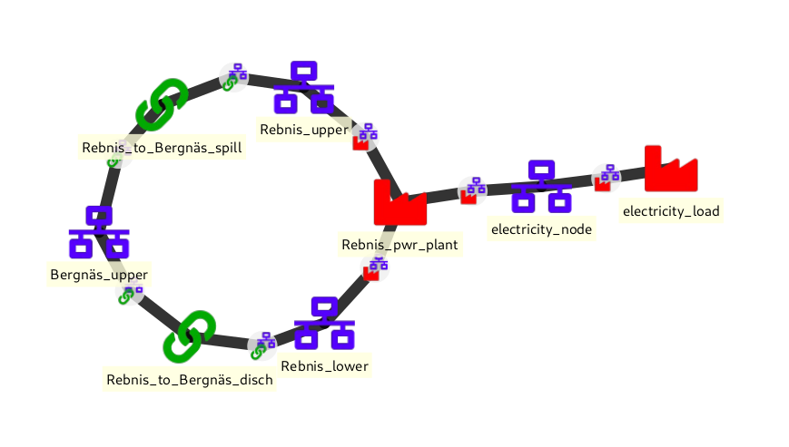
On the contrary, the model of the river system is more detailed. Each power station in the river is modelled using the following elements:
- An upper water node, located at the entrance of the station.
- A lower water node, located at the exit of the station.
- A power plant unit, that discharges water from the upper node into the lower node, and feeds electricity produced in the process to the common electricity node.
- A spillway connection, that takes spilled water from the upper node and releases it to the downstream upper node.
- A discharge connection, that takes water from the lower node and releases it to the downstream upper node.
Below is a schematic of the model. For clarity, only the Rebnis station is presented in full detail:
In order to run this tutorial you must first execute some preliminary steps from the Simple System tutorial. Specifically, execute all steps from the guide, up to and including the step of importing the spineopt database template. It is advisable to go through the whole tutorial in order to familiarise yourself with Spine.
Just remember to give a different name for the Spine Project of the hydropower tutorial (e.g., ‘Case Study A5’) in the corresponding step, so to not mix up the Spine Toolbox projects!
Importing the SpineOpt database template
- Download the SpineOpt database template (right click on the link, then select Save link as...)
- Select the input Data Store item in the Design View.
- Go to Data Store Properties and hit Open editor. This will open the newly created database in the Spine DB Editor, looking similar to image below.
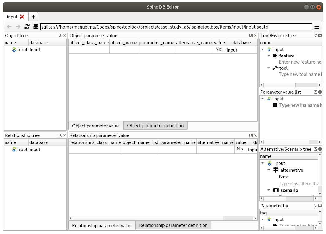
The Spine DB editor is a dedicated interface within Spine Toolbox for visualizing and managing Spine databases.
- Press Alt + F to display the editor menu, select File -> Import..., and then select the template file you previously downloaded (in case it is not displayed in the folder where you saved it, double-check that you selected). The contents of that file will be imported into the current database, and you should then see classes like ‘commodity’, ‘connection’ and ‘model’ under the root node in the Object tree (on the left).
- From the editor menu (Alt + F), select Session -> Commit. Enter ‘Import SpineOpt template’ as message in the popup dialog, and click Commit.
The SpineOpt template contains the fundamental object and relationship classes, as well as parameter definitions, that SpineOpt recognizes and expects. You can think of it as the generic structure of the model, as opposed to the specific data for a particular instance. In the remainder of this section, we will add that specific data for the Skellefte river.
Entering data
There are two options in this tutorial to enter data in the Database. The first one is to enter data manually and the second to use the importer functionality. These are described in the next two subsections respectively and produce similar models. The model created when using the importer creates a model with two-segments efficiency curves for converting water to electricity (while the model created when entering the data manually assumes a simplified efficiency curve with a single segment).
Entering data manually
Creating objects
To add power plants to the model, stay in the Spine DB Editor and create objects of class
unitas follows:- Select the list of plant names from the text-box below and copy it to the clipboard (Ctrl+C)
Rebnis_pwr_plant Sadva_pwr_plant Bergnäs_pwr_plant Slagnäs_pwr_plant Bastusel_pwr_plant Grytfors_pwr_plant Gallejaur_pwr_plant Vargfors_pwr_plant Rengård_pwr_plant Båtfors_pwr_plant Finnfors_pwr_plant Granfors_pwr_plant Krångfors_pwr_plant Selsfors_pwr_plant Kvistforsen_pwr_plant - Go to Object tree (on the top left of the window, usually), right-click on
unitand select Add objects from the context menu. This will open the Add objects dialog. - Select the first cell under the object name column and press Ctrl+V. This will paste the list of plant names from the clipboard into that column; the object class name column will be filled automatically with ‘unit‘. The form should now be looking similar to this:
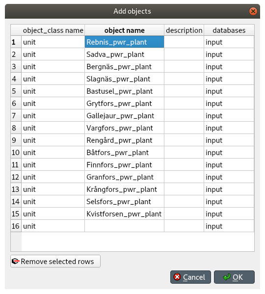
- Click Ok.
- Back in the Spine DB Editor, under Object tree, double click on
unitto confirm that the objects are effectively there. - Commit changes with the message ‘Add power plants’.
- Select the list of plant names from the text-box below and copy it to the clipboard (Ctrl+C)
Add discharge and spillway connections by creating objects of class
connectionwith the following names:RebnistoBergnäsdisch SadvatoBergnäsdisch BergnästoSlagnäsdisch SlagnästoBastuseldisch BastuseltoGrytforsdisch GrytforstoGallejaurdisch GallejaurtoVargforsdisch VargforstoRengårddisch RengårdtoBåtforsdisch BåtforstoFinnforsdisch FinnforstoGranforsdisch GranforstoKrångforsdisch KrångforstoSelsforsdisch SelsforstoKvistforsendisch Kvistforsentodownstreamdisch RebnistoBergnässpill SadvatoBergnässpill BergnästoSlagnässpill SlagnästoBastuselspill BastuseltoGrytforsspill GrytforstoGallejaurspill GallejaurtoVargforsspill VargforstoRengårdspill RengårdtoBåtforsspill BåtforstoFinnforsspill FinnforstoGranforsspill GranforstoKrångforsspill KrångforstoSelsforsspill SelsforstoKvistforsenspill Kvistforsentodownstreamspill
Add water nodes by creating objects of class
nodewith the following names:Rebnisupper Sadvaupper Bergnäsupper Slagnäsupper Bastuselupper Grytforsupper Gallejaurupper Vargforsupper Rengårdupper Båtforsupper Finnforsupper Granforsupper Krångforsupper Selsforsupper Kvistforsenupper Rebnislower Sadvalower Bergnäslower Slagnäslower Bastusellower Grytforslower Gallejaurlower Vargforslower Rengårdlower Båtforslower Finnforslower Granforslower Krångforslower Selsforslower Kvistforsenlower
Next, create the following objects (all names in lower-case):
instanceof classmodel.waterandelectricityof classcommodity.electricity_nodeof classnode.electricity_loadof classunit.some_weekof classtemporal_block.deterministicof classstochastic_structure.realizationof classstochastic_scenario.
Finally, create the following objects to get results back from SpineOpt (again, all names in lower-case):
my_reportof classreport.unit_flow,connection_flow, andnode_stateof classoutput.
To modify an object after you enter it, right click on it and select Edit... from the context menu.
Specifying object parameter values
To specify the general behaviour of our model, stay in the Spine DB Editor and enter model parameter values as follows:
- Select the model parameter value data (i.e. select all, Ctrl+A) from the file below and copy it to the clipboard (Ctrl+C): cs-a5-model-parameter-values.txt
- Select
instancein the Object tree and inspect the table in Object parameter value (on the top-center of the window, usually). Make sure that the columns in the table are ordered as follows (drag and drop columns if you need to change their order):
object_class_name | object_name | parameter_name | alternative_name | value | database- Select the first cell under
object_class_nameand press Ctrl+V. This will paste the model parameter value data from the clipboard into the table. The form should be looking like this: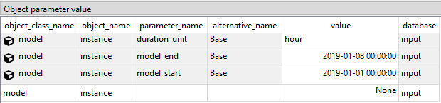
Specify the resolution of our temporal block
some_weekin the same way using the data below: cs-a5-temporal_block-parameter-values.txtSpecify the behaviour of all system nodes with the data below, where:
demandrepresents the local inflow (negative in most cases).fix_node_staterepresents fixed reservoir levels (at the beginning and the end).has_stateindicates whether or not the node is a reservoir (true for all the upper nodes).state_coeffis the reservoir 'efficienty' (always 1, meaning that there aren't any loses).node_state_capis the maximum level of the reservoirs.
To do this in one single step, simply select
nodein the Object tree and paste the following values in the first empty cell: cs-a5-node-parameter-values.txt
Establishing relationships
To enter the same text on several cells, copy the text into the clipboard, then select all target cells and press Ctrl+V.
Create relationships of the class
unit__from_nodeto represent that a power plant receives water from the station's upper water node, and that the electricity load takes electricity from the common electricity node. Both the power plants and the electricity load belong to the classunit.- Select the list of unit and node names from below and copy it to the clipboard (Ctrl+C). cs-a5-unit__from_node.txt
- In the Spine DB Editor, go to Relationship tree (on the bottom left of the window, usually), right-click on
unit__from_nodeand select Add relationships from the context menu. This will open the Add relationships dialog. - Select the first cell under the unit column and press Ctrl+V. This will paste the list of plant and node names from the clipboard into the table. The form should be looking like this:
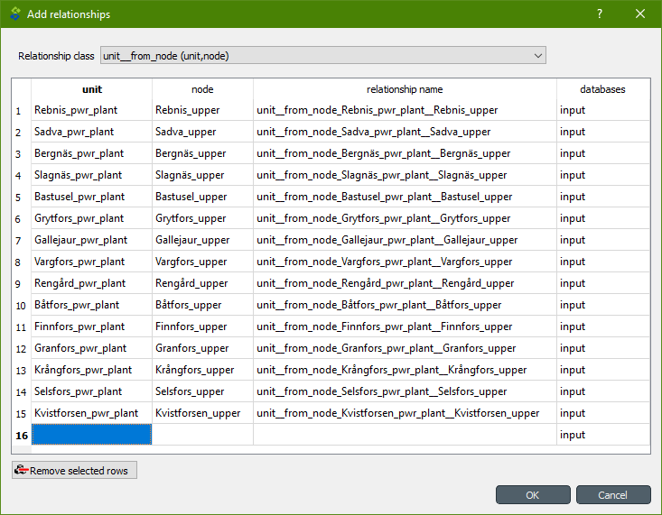
- Click Ok.
- Back in the Spine DB Editor, under Relationship tree, double click on
unit__from_nodeto confirm that the relationships are effectively there. - From the main menu (Alt + F), select Session -> Commit to open the Commit changes dialog. Enter ‘Add from nodes of power plants‘ as the commit message and click Commit.
Create relationships of the class
unit__to_nodeto represent that a power plant releases water to the station's lower water node, and that the power plants supply electricity to the common electricity node. Use the following data and do as before: cs-a5-unit__to_node.txt
At this point, you might be wondering what's the purpose of the unit__node__node relationship class. Shouldn't it be enough to have unit__from_node and unit__to_node to represent the topology of the system? The answer is yes; but in addition to topology, we also need to represent the conversion process that happens in the unit, where the water from one node is turned into electricty for another node. And for this purpose, we use a relationship parameter value on the unit__node__node relationships (see Specifying relationship parameter values).
Create relationships of the class
connection__from_nodeto represent that water can be either discharged or spilled. If discharged, it is taken from the lower water node of the station, if spilled it is taken from the upper water node of the station. Use the following data and do as before: cs-a5-connection__from_node.txtCreate relationships of the class
connection__to_nodeto represent that both discharge and spill are released into the upper node of the next downstream station. Use the following data and do as before: cs-a5-connection__to_node.txt
At this point, you might be wondering what's the purpose of the connection__node__node relationship class. Shouldn't it be enough to have connection__from_node and connection__to_node to represent the topology of the system? The answer is yes; but in addition to topology, we also need to represent the delay in the river branches. And for this purpose, we use a relationship parameter value on the connection__node__node relationships (see Specifying relationship parameter values).
Create relationships of the class
node__commodityto represent that each node has to be in balance, for water nodes with respect to water, for electricity nodes with respect to electricity. This way, you link all nodes to either the commocitywateror the commodityelectricity. Use the following data and do as before: cs-a5-node__commodity.txtDefine that all nodes in our model have to be balanced at each time step. To do this, you create a relationship of the class
model__default_temporal_blockbetween the modelinstanceand the temporalblock `someweek` in the same way as before.Define that our model is deterministic. To do this, you create a relationship of the class
model__default_stochastic_structurebetween the modelinstanceand the stochastic structuredeterministic, as well as a relationship of classstochastic_structure__stochastic_scenariobetween the stochastid structuredeterministicand the stochastic scenariorealizationin the same way as before.In order to get the results from running Spine Opt written to the ouput database, create relationships of the class
report__outputbetween the reportmy_reportand each of the followingoutputobjects:unit_flow,connection_flow, andnode_state. In addition, you also need to create a relationship of the classmodel__reportbetween the modelinstanceand the reportmy_report.
Specifying parameter values of the relationships
Finally, the values of all parameters have to be entered. Specify the capacity of all hydropower plants, and their respective variable operating cost by entering
unit__from_nodeparameter values as follows:- Select the data from the text-box below and copy it to the clipboard (Ctrl+C): cs-a5-unit__from_node-relationship-parameter-values.txt
- In the Spine DB Editor, go to Relationship tree (on the bottom left of the window, usually), and click on
unit__from_node. Then, go to Relationship parameter value (on the bottom-center of the window, usually). Make sure that the columns in the table are ordered as follows (drag and drop columns if you need to change their order):
relationship_class_name | object_name_list | parameter_name | alternative_name | value | database- Select the first cell under
relationship_class_nameand press Ctrl+V. This will paste the parameter value data from the clipboard into the table.
Specify the conversion ratio between discharged water and generated electricity for each hydropower station as well as a similar conversion rate (set to 1) to represent that water cannot be lost between upper and lower water nodes. Use the following data to enter the parameter values
unit__from_node: cs-a5-unit__node__node-relationship-parameter-values.txtSpecify the average discharge and spillage in the first hours of the simulation. Use the following data to enter the parameter values
connection__from_node: cs-a5-connection__from_node-relationship-parameter-values.txtFinally, specify the delay (the time it takes for the water to run between water nodes) and the transfer ratio (being equal to 1) of different water connections. Use the following data to enter the parameter values
connection__node_node: cs-a5-connection__node__node-relationship-parameter-values.txtWhen you're ready, commit all changes to the database via the main menu (Alt + F).
Using the Importer
Additional Steps for Project Setup
- Drag the Data Connection icon
 from the tool bar and drop it into the Design View. This will open the Add Data connection dialogue. Type in ‘Data Connection’ and click on Ok.
 - To import the model into the Spine database, you need to create an Import specification. Create an Import specification by clicking on the small arrow next to the Importer item (in the Main section of the toolbar) and press New. The Importer specification editor will pop-up.
- Type ‘Import Model’ as the name of the specification. Save the specification by using Ctrl+S and close the window.
- Drag the newly created Import Model Importer item icon
 from the tool bar and drop it into the Design View. This will open the Add Importer dialogue. Type in ‘Import Model’ and click on Ok.
 - Connect ‘Data Connection’ with ‘Import Model’ by first clicking on one of the Data Connection’s connectors and then on one of the Importer’s connectors. Connect similarly the importer with the input database. Now the project should look similar to this:
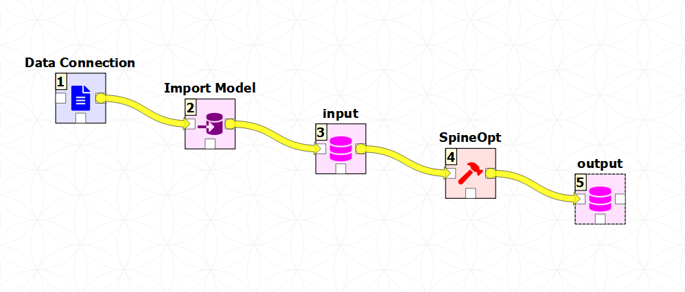
- From the main menu, select File -> Save project.
Importing the model
- Download the data and the accompanying mapping (right click on the links, then select Save link as...).
- Add a reference to the file containing the model.
- Select the Data Connection item in the Design View to show the Data Connection properties window (on the right side of the window usually).
- In Data Connection Properties, click on , click on the icon furthest to the left Add file references and select the previously downloaded Excel file.
- Next, double click on the Import model in the Design view. A window called Select connector for Import Model will pop-up, select Excel and klick OK. Next, still in the Importer specification editor, click on the main menu icon in the top right (or Press Alt + F to automatically display it) and import the mappings previously downloaded (by clicking on Import mappings). Finally, save by clicking Ctrl+S and exit the Importer specification editor.
Executing the workflow
Once the workflow is defined and input data is in place, the project is ready to be executed. Hit the Execute project button  on the tool bar.
You should see ‘Executing All Directed Acyclic Graphs’ printed in the Event log (on the lower left by default). SpineOpt output messages will appear in the Process Log panel in the middle. After some processing, ‘DAG 1/1 completed successfully’ appears and the execution is complete.
Examining the results
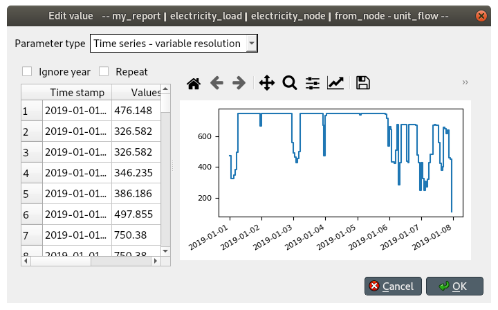
Select the output data store and open the Spine DB editor.
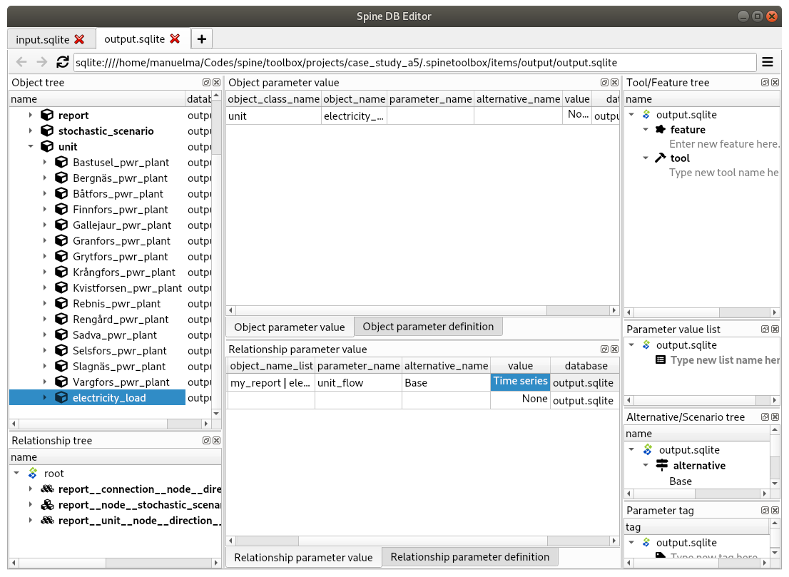
To checkout the flow on the electricity load (i.e., the total electricity production in the system), go to Object tree, expand the unit object class, and select electricity_load, as illustrated in the picture above. Next, go to Relationship parameter value and double-click the first cell under value. The Parameter value editor will pop up. You should see something like this:
If you have used the importer to instantiate the model you can easily modify the parameters in the model worksheet, run the project and observe the differences in the results. If you need to make changes directly to the input database, in order for the importer not to overwrite them, you will need to dissassociate the importer from the input DB (right click in the connecting yellow arrow between the two items and click on remove).