Ramping definition tutorial
This tutorial provides a step-by-step guide to include ramping constraints in a simple energy system with Spine Toolbox for SpineOpt.
Introduction
Welcome to our tutorial, where we will walk you through the process of adding ramping constraints in SpineOpt using Spine Toolbox. To get the most out of this tutorial, we suggest first completing the Simple System tutorial, which can be found here.
The ramping constraint limit refers to the maximum rate at which a power unit can increase or decrease its output flow over time. These limits are typically put in place to prevent sudden and destabilizing shifts in power units. However, they may also represent any other physical limitations that a unit may have that is related to changes over time in its output flow.
Model assumptions
This tutorial is built on top of the Simple System. The main changes to that system are:
- The demand at electricity_node is a 3-hour time series instead of a unique value
- The power_plant_a has the following parameters:
- Ramp limit of 10% for both up and down
- Minimum operating point of 10% of its total capacity
- Startup capacity limit of 10% of its total capacity
- Shutdown capacity limit of 10% of its total capacity
This tutorial includes a step-by-step guide to include the parameters to help analyze the results in SpineOpt and the ramping constraints concepts.
Step 1 - Update the demand
Opening the Simple System project
- Launch the Spine Toolbox and select File and then Open Project or use the keyboard shortcut Alt + O to open the desired project.
- Locate the folder that you saved in the Simple System tutorial and click Ok. This will prompt the Simple System workflow to appear in the Design View section for you to start working on.
- Select the 'input' Data Store item in the Design View.
- Go to Data Store Properties and hit Open editor. This will open the database in the Spine DB editor.
In this tutorial, you will learn how to add ramping constraints to the Simple System using the Spine DB editor, but first let's start by updating the electricity demand from a single value to a 3-hour time series.
Editing demand value
- Always in the Spine DB editor, locate the Object tree (typically at the top-left). Expand the [root] element if not expanded.
- Expand the node class, and select the electricity_node from the expanded tree.
- Locate the Object parameter table (typically at the top-center).
- In the Object parameter table, identify the demand parameter which should have a 150 value from the Simple System first run.
- Right-click on the value cell and then select edit from the context menu. The Edit value dialog will pop up.
- Change the Parameter type to Time series fixed resolution, resolution to 1h, and the demand values to the time series as in the image below.
- Finish by pressing OK in the Edit value menu. In the Object parameter table you will see that the value of the demand has changed to Time series.
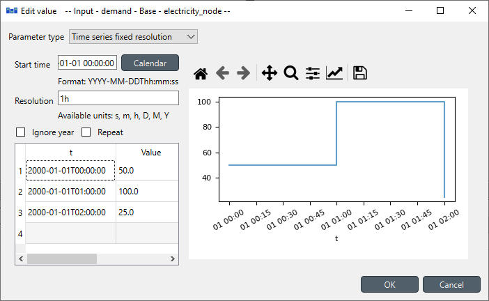
Notice that there is only demand values for 2000-01-01T00:00:00 and 2000-01-01T02:00:00. Therefore, we need to update the start and end of the model. But first, let's change the temporal block.
Editing the temporal block
You might or might not notice that the Simple System has, by default, a temporal block resolution of 1D (i.e., one day); wait, what! Yes, by default, it has 1D in its template. So, we want to change that to 1h to make easy to follow the results.
- Locate again the Object tree (typically at the top-left). Expand the [root] element if not expanded.
- Expand the model class, and select the simple from the expanded tree.
- Locate the Object parameter table (typically at the top-center).
- In the Object parameter table, identify the resolution parameter which should have a 1D value from the Simple System first run.
- Right-click on the value cell and then select edit from the context menu. The Edit value dialog will pop up.
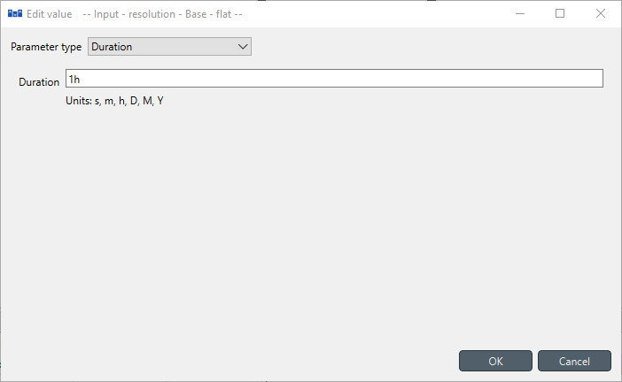
- Change the Duration from 1D to 1h as shown in the image below.
Editing the model start and end
Since the default resolution of the Simple System was 1D, the start and end date of the model needs also to be changed.
- Locate again the Object tree (typically at the top-left). Expand the [root] element if not expanded.
- Expand the temporal_block class, and select the flat from the expanded tree.
- Locate the Object parameter table (typically at the top-center).
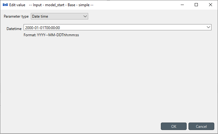
- In the Object parameter table, select the model_start parameter, the Base alternative, and then right-click on the value and select the Edit option in the context menu, as shown in the image below.
- Repeat the procedure for the model_end parameter, but now the value is
2000-01-01T03:00:00. The final values should look like that the image below.
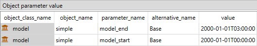
It's important to note that the model must finish in the third hour to account for all the periods of demand in input data, which goes until
2000-01-01T02:00:00.
When you're ready, save/commit all changes to the database.
Executing the workflow
Go back to Spine Toolbox's main window, and hit the Execute project button from the toolbar. You should see 'Executing All Directed Acyclic Graphs' printed in the Event log (at the bottom left by default).
Select the 'Run SpineOpt' Tool. You should see the output from SpineOpt in the Julia Console after clicking the object activity control.
Examining the results
Select the output data store and open the Spine DB editor. You can already inspect the fields in the displayed tables or use a pivot table.
For the pivot table, press Alt + F for the shortcut to the hamburger menu, and select Pivot -> Index.
Select
report__unit__node__direction__stochastic_scenariounder Relationship tree, and the first cell under alternative in the Frozen table.Under alternative in the Frozen table, you can choose results from different runs. Pick the run you want to view. If the workflow has been run several times, the most recent run will usually be found at the bottom.
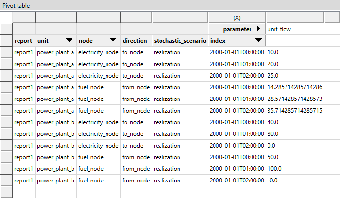
The Pivot table will be populated with results from the SpineOpt run. It will look something like the image below.
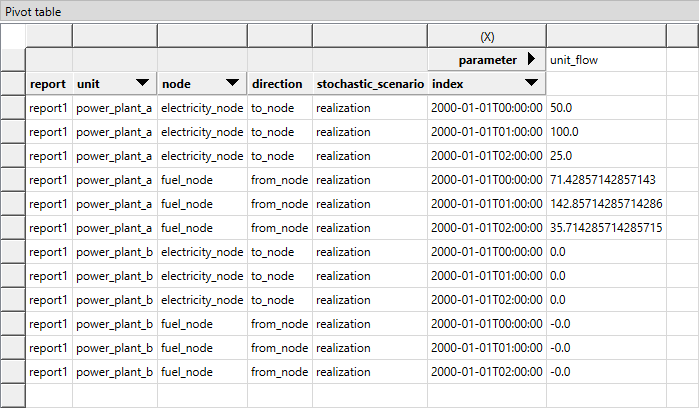
The image above shows the electricity flow results for both power plants. As expected, the power_plant_a (i.e., the cheapest unit) always covers the demand in both hours, and then the power_plant_b (i.e., the more expensive unit) has zero production. This is the most economical dispatch since the problem has no extra constraints (so far!).
Step 2 - Include the ramping limit
Let's consider the input data where the power_plant_a has a ramping limit of 10% in both directions (i.e., up and down), meaning that the change between two time steps can't be greater than 10MW (since the plant 'a' has a unit capacity of 100MW). The ramping constraints need the following parameters for their definition: minimum operating point, startup limit, and shutdown limit. For more details, please visit the mathematical formulation in the following link
Adding the new parameters
In Relationship tree, expand the unit__to_node class and select power_plant_a | electricity_node.
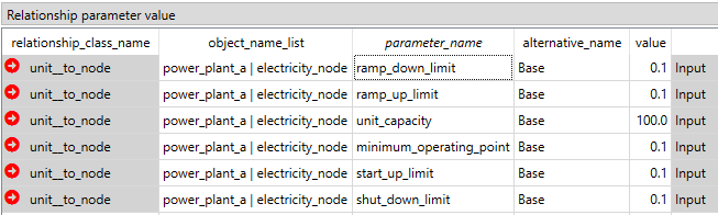
In the Relationship parameter table:
Select the ramp_limits_up parameter and the Base alternative, and enter the value 0.1 as seen in the image below. This will set the ramping up limit for power_plant_a.
Select the ramp_limits_down parameter and the Base alternative, and enter the value 0.1 as seen in the image below. This will set the ramping down limit for power_plant_a.
Select the minimum_operating_point parameter and the Base alternative, and enter the value 0.1 as seen in the image below. This will set the minimum operating point for power_plant_a.
Select the ramp_limits_startup parameter and the Base alternative, and enter the value 0.1 as seen in the image below. This will set the startup capacity limit for power_plant_a.
Select the ramp_limits_shutdown parameter and the Base alternative, and enter the value 0.1 as seen in the image below. This will set the shutdown capacity limit for power_plant_a.
When you're ready, save/commit all changes to the database.
Executing the workflow with ramp limits
Go back to Spine Toolbox's main window, and hit the Execute project button from the toolbar. You should see 'Executing All Directed Acyclic Graphs' printed in the Event log (at the bottom left by default).
Select the 'Run SpineOpt' Tool. You should see the output from SpineOpt in the Julia Console after clicking the object activity control.
Examining the results with ramp limits
Select the output data store and open the Spine DB editor. You can already inspect the fields in the displayed tables or use a pivot table.
For the pivot table, press Alt + F for the shortcut to the hamburger menu, and select Pivot -> Index.
Select
report__unit__node__direction__stochastic_scenariounder Relationship tree, and the first cell under alternative in the Frozen table.Under alternative in the Frozen table, you can choose results from different runs. Pick the run you want to view. If the workflow has been run several times, the most recent run will usually be found at the bottom.
The Pivot table will be populated with results from the SpineOpt run. It will look something like the image below.
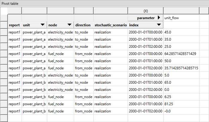
The image above shows the electricity flow results for both power plants. As expected, the power_plant_a (i.e., the cheapest unit) output is limited to its ramps limits, therefore it can't follow the demand changes as before. For instance, the unit's power output is 45MW in the first hour, which is lower than the previous result of 50MW in the same hour. This is because the unit needs to gradually decrease its power output and reach 25MW in the last hour. However, due to the imposed ramp-down limit of 10MW, it cannot start from 50MW as before. Therefore, the power_plant_b (i.e., the more expensive unit) must produce to cover the demand that plant 'a' can't due to its ramping limitations. As shown here, the ramping limits might lead to higher costs in power systems compared to the previous case.
But...there is something more here...Can you tell what? :anguished:
It is important to note that the optimal solution we have calculated assumes that the unit 'a' was already producing electricity before the model_start parameter. This is because we have not defined an initial condition for the flow of the unit. Therefore, the flow at the first hour is the most cost-effective solution under this assumption. However, what if we changed this assumption and assumed that the unit had not produced any flow before the model_start parameter? If you are curious to know the answer, join me in the next section.
Step 3 - Include a initial condition to the flow
Adding the initial flow
In Relationship tree, expand the unit__to_node class and select power_plant_a | electricity_node.
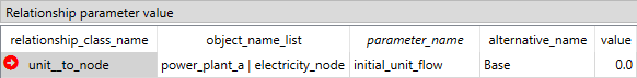
In the Relationship parameter table, select the flow_limits_initial parameter and the Base alternative, and enter the value 0.0 as seen in the image below. This will set the initial flow for power_plant_a.
When you're ready, save/commit all changes to the database.
Executing the workflow with ramp limits with initial conditions
You know the drill! ;)
Examining the results with ramp limits with initial conditions
Create a Pivot table with the latest results. It will look something like the image below.
Here, we can see the impact of the initial condition; no longer can the unit have a flow change than its ramp-up limit for the first hour. Therefore, the optimal solution under this assumption changes compared to the previous section.
This example highlights the importance of considering initial conditions as a crucial assumption in energy system modelling optimization.