Multi-year Investments Using Economic Parameters Tutorial
The basics of how to set up a capacity planning model are covered in Capacity Planning Tutorial and multi-year investments in Multi-year investments. With that information, you should be able to do multi-year investments already with your own parameters. However, the correct representation for costs across years can be tricky. To make it more user-friendly, SpineOpt has incorporated some pre-defined economic parameters internally, and the goal of this tutorial is to walk you through the set-up for using these parameters.
Overview
In this tutorial, we will
- simplify the simple system tutorial by only using one
power_plant, - show the necessary parameters to activate and use pre-defined internal parameters,
- show you how to use these economic parameters,
- show you how to use milestone years.
Set-up
To avoid repetition, we only consider one unit instead of the two units from the simple system tutorial. The easiest way to do this is to import the simple system (file > import) and to remove one of the two power plants. To remove a power plant, right-click power_plant_b in the Entity tree and select Remove.... This also removes the entities that refer to power_plant_b (e.g. fuel_node | power_plant_b) and their parameter values, but not the nodes, which we still need for power_plant_a. There will be a confirmation box with an overview of all the entities that you will be removing.
Since we are working with investments, we are going to make a distinction between investments and operation in the time blocks. We retain the original time block, rename it from flat to operation and adjust the resolution to 4 months ('4M'). Additionally, we add an investment time block with a resolution of 5 years ('5Y') between 2000 and 2006. We have to adjust the time horizon of the model entity accordingly. As in the Capacity Planning Tutorial, connect the investment time block to the model with the model__default_investment_temporal_block entity, and the existing stochastic structure with the model__default_investment_stochastic_structure entity.
Once we have our setup, we can take a look at the economic representation in SpineOpt. Below is a list of parameters you would need:
- multiyear_economic_discounting: activation value in a choice between
consecutive_yearsandmilestone_years, with the default value beingnull(Nonein a SpineDB andnothingin Julia). When a valid value is selected, the model will use its internally-calculated parameters for discounting investment and operation costs. Specifically, choosingconsecutive_yearsrequires the model to use continuous operational temporal blocks, and thus the operation cost will be discounted every year. In contrast, choosingmilestone_yearsmeans the model will discount the operation cost as per the investment temporal block. - discount_rate: the rate you would like to discount your costs with.
- discount_year: the year you would like to discount your costs to.
- lifetime_technical: using units as an example, this is the technical lifetime of the unit.
- lifetime_economic: using units as an example, this is the economic lifetime of the unit which is used to calculate the economic parameters.
- [optional] discount_rate_technology_specific: using units as an example, this is used if you would like to have a specific discount rate different from discount_rate.
- [optional] lead_time: if not specified, the default lead time is 0.
- unit_investment_cost: using unit as an example, this is the investment cost for the investment year. When multiyear_economic_discounting is not used (i.e. with the default value
null), then this cost that you put will not be discounted at all. However, when you choose a valid value of multiyear_economic_discounting, SpineOpt will discount this cost to the discount_year using discount_rate.
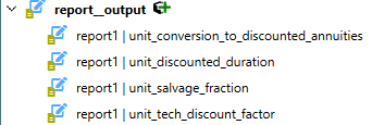
To be able to see the values of the economic parameters after a run, you have to add them to the report.
Not using economic discounting
We start with the case where multiyear_economic_discounting is not used with the default value null, which means SpineOpt will not create and use its internally-calculated parameters for discounting investment and operation costs. A unit_investment_cost of 100 and a vom_cost of 25 are not discounted at all. See the set-up below (the parameter values with alternative Base; the values that come with the simple system are marked with *).
In the Entity tree, select root. Among the values in the Parameter value table, you should see:
| group | class | entity byname | parameter name | alternative | value |
|---|---|---|---|---|---|
| model | simple | discount_rate | Base | 0.05 | |
| model | simple | discount_year | Base | 1990-01-01T00:00:00 | |
| model | simple | model_start | Base | 2000-01-01T00:00:00 | |
| model | simple | model_end | Base | 2006-01-01T00:00:00 | |
| node | electricity_node | demand | Base | 100.0 | |
| node | fuel_node | balance_type | Base | none * | |
| temporal_block | investment | block_start | Base | 2000-01-01T00:00:00 | |
| temporal_block | investment | block_end | Base | 2006-01-01T00:00:00 | |
| temporal_block | investment | resolution | Base | 5Y | |
| temporal_block | operation | resolution | Base | 4M | |
| unit | power_plant_a | existing_units | Base | 0.0 | |
| unit | power_plant_a | investment_count_max_cumulative | Base | 1.0 | |
| unit | power_plant_a | discount_rate_technology_specific | Base | 0.07 | |
| unit | power_plant_a | unit_investment_cost | Base | 100.0 | |
| unit | power_plant_a | lifetime_economic | Base | 10Y | |
| unit | power_plant_a | lifetime_technical | Base | 10Y | |
| node__to_unit | fuel_node ǀ power_plant_a | vom_cost | Base | 25.0 * | |
| unit__to_node | power_plant_a ǀ electricity_node | capacity_per_unit | Base | 100.0 * | |
| unit_flow__unit_flow | power_plant_a ǀ electricity_node ǀ fuel_node ǀ power_plant_a | flow_ratio_equality_coefficient | Base | 1.0 |
Note that existing_units is set to 0, since its default value is 1 and the model would otherwise not need to invest.
Using economic parameters with consecutive operation years
Now we set multiyear_economic_discounting to consecutive_years. This set-up indicates that the model will use the internally-calculated parameters and continuous operational temporal blocks. Now the unit_investment_cost and the vom_cost are discounted to 1990 using a discount_rate of 0.05. Compared to the previous set-up, we only add one value:
In the Entity tree, expand model and select simple. The Parameter value table should show:
| group | class | entity byname | parameter name | alternative | value |
|---|---|---|---|---|---|
| model | simple | multiyear_economic_discounting | Base | consecutive_years |
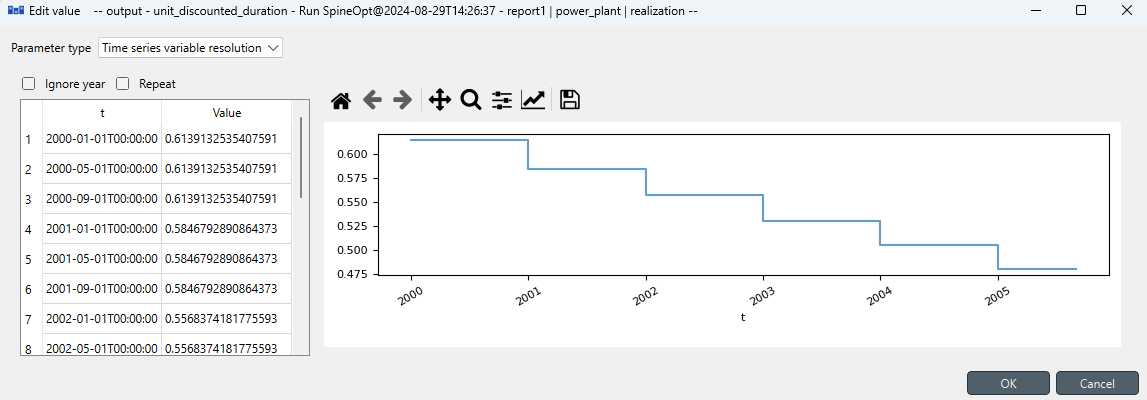
The values for the output parameter unit_discounted_duration are shown below. It is used to discount operation costs so it has the resolution of the operational temporal block. However, since we only discount per year, this parameter value is constant within a year.
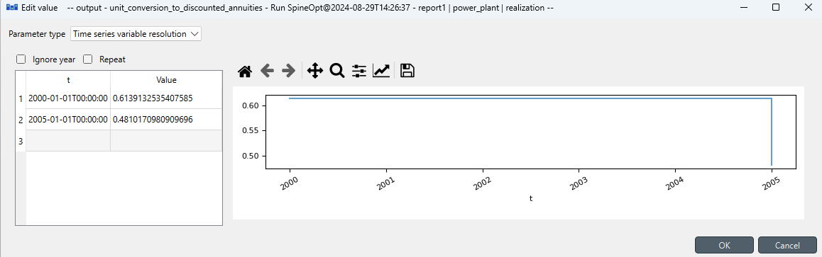
The rest is for discounting investment costs with the resolution of the investment temporal block.
Using economic parameters with milestone investment years
Now we set multiyear_economic_discounting to milestone_years. This indicates that we want operational temporal block to be discontinuous and use the same milestone years as the investment temporal block. In this case, we need to change the definition of temporal blocks. Compared to the previous set-up, set multiyear_economic_discounting to milestone_years, delete the operation temporal block and add two new operation temporal blocks, both connected to the model with model__default_temporal_block entities (simple | operation1 and simple | operation2):
In the Entity tree, select root. Among the values in the Parameter value table, you should now see:
| group | class | entity byname | parameter name | alternative | value |
|---|---|---|---|---|---|
| model | simple | multiyear_economic_discounting | Base | milestone_years | |
| temporal_block | operation1 | block_start | Base | 2000-01-01T00:00:00 | |
| temporal_block | operation1 | block_end | Base | 2001-01-01T00:00:00 | |
| temporal_block | operation1 | resolution | Base | 4M | |
| temporal_block | operation2 | block_start | Base | 2004-09-01T00:00:00 | |
| temporal_block | operation2 | block_end | Base | 2006-01-01T00:00:00 | |
| temporal_block | operation2 | resolution | Base | 4M | |
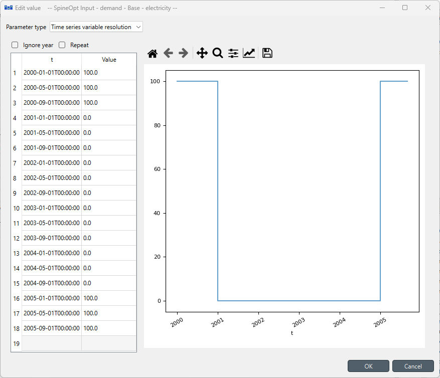
| node | electricity_node | demand | Base | Time series (see below) |
where the demand TimeSeries is defined as follows: