Stochastic structure tutorial
Welcome to Spine Toolbox's Stochastic System tutorial.
This tutorial provides a step-by-step guide to get started with the stochastic structure. More information can be found in the documentation on the stochastic structure. It is recommended to make sure you are able to get the simple system tutorial working first.
In this tutorial we will take a look at independent scenarios and stochastic paths.
In theory it is also possible to have different stochastic structures in different parts of your system. In practice that is very much prone to errors. As much of the functionality of different stochastic structures can be accomplished with a clever DAG, it is recommended to work with a single stochastic structure at all times.
Setup starting from simple system tutorial
We create a new Spine Toolbox project and start from the simple system tutorial.
For the Spine Toolbox project
- Open Spine Toolbox
- Create a new Spine Toolbox project
- Add two data store items (input and output)
- set the dialect to
sqlite - push the new database button
- set the dialect to
- Add the run SpineOpt tool
- connect the databases to the SpineOpt tool
- in the properties pane of the SpineOpt tool,
For the simple system tutorial
- Download the simple system database (
jsonfile)
from the ./examples/ folder in the SpineOpt repository (you can save the json file in your Spine Toolbox project folder)
- Enter the input database such that you are in the spine DB editor
- Go to the hamburger menu (Alt+F) and select import
- Locate the downloaded file to import the simple system
- We save our results when we commit to the database,
so go again to the hamburger menu and select commit. The update message can be something like this: import simple system tutorial.
The graph view is not always enabled by default. If you want to see the simple system, go to the hamburger menu and select graph.
Independent scenarios
Recall from the simple system tutorial that there actually already is a stochastic structure present. Let us take a closer look at that structure.
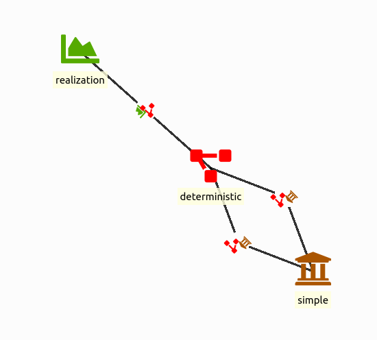
The scenarios are the labels that are available to the user to label their data. Don't worry, we'll come back to that later. Here, there is currently one scenario realization.
The stochastic_scenarios are managed by the stochastic_structures. The stochastic_structures are connected to different parts of the energy system to manage them. With the model__default_stochastic_structure relationship we can connect a stochastic_scenario to the entire energy system. Here, there is one stochastic_structure deterministic which is also the systems default.
It is quite simple to add an independent stochastic_scenario to this existing stochastic_structure.
- Add a stochastic_scenario object and call it independent
- Add a stochastic_structure__stochastic_scenario relationship between independent and deterministic
either from the tree view (right-click -> new relationship) or from the graph view (right-click -> add relationship)
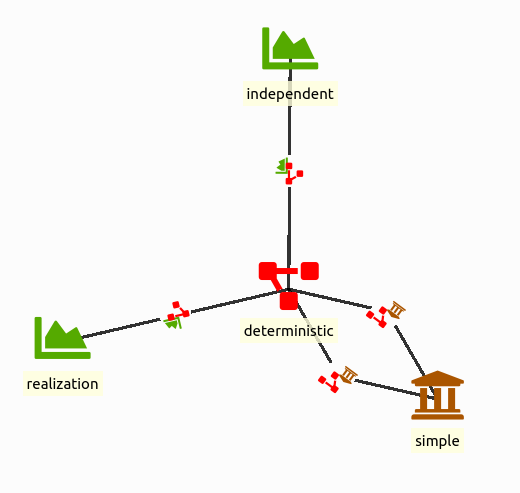
Now we can use these labels in the values for the energy system.
- Change the demand parameter at the electricity_node from 150.0 to a map
(right-click -> edit, parameter type map)
- for the x column we can use our stochastic_scenario labels, for the Value column we can choose our values
- Choose realization 150.0 and independent 100.0
- Save/Commit the results
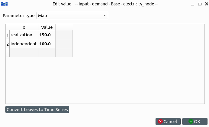
That is it! We can now run the model and the output database will show the results for both stochastic_scenarios. In the realization stochastic_scenario power plant b produces an output of 50. In the independent stochastic_scenario power plant b does not produce anything as the demand is low enough for power plant a to produce all the necessary energy.
Stochastic path
SpineOpt always works with stochastic paths. The stochastic path describes which stochastic_scenarios are active at each time step. The stochastic_structure collects the stochastic paths in a direct acyclic graph (DAG).
But let's make that more clear with an example. We can continue from the previous structure, but let's rename the stochastic_structure and stochastic_scenario. (optional step)
- Right-click the object (either in the tree view or the graph view) and select edit
- Rename the stochastic_structure from deterministic to DAG
- Rename the realization stochastic_scenario to base
- Rename the independent stochastic_scenario to forecast1
Perhaps from the name you already guessed it, we are going to add some stochastic_scenarios.
- Add two stochastic_scenario objects forecast2 and forecast3
- Connect the two stochastic_scenarios to stochastic_structure
And we need to adjust the Map for the electricity demand accordingly.
- Edit the
Mapand provide a value for each stochastic_scenario
(see image below)
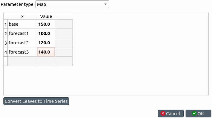
All these stochastic_scenario are independently available to the stochastic_structure, but now we want to define the underlying relationships to make a stochastic path. In particular, we want to start from a base stochastic_scenario and later split into the forecast stochastic_scenario. For SpineOpt, that means that the base stochastic_scenario is the parent, and the following forecast stochastic_scenarios are its children.
for each forecast stochastic_scenario and select the base stochastic_scenario as its parent (the first stochastic_scenario is the parent and the second stochastic_scenario is its child)
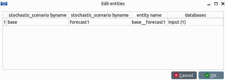
We also need to tell SpineOpt what the probability is that we end up in a certain child. That information is stored in the stochastic_structure so you'll find the corresponding parameter in the stochastic_structure__stochastic_scenario relationship. Here we assume that each forecast is equally likely to happen.
- for each DAG | forecast relationship, add a value for
the weight_relative_to_parents parameter; the sum needs to be equal to 1

That results in the stochastic_structure below.
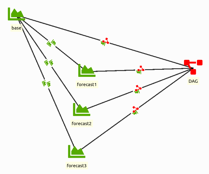
We can run the SpineOpt tool on this database, but we will only see the values for the base stochastic_scenario. That is because SpineOpt assumes that a stochastic_scenario runs forever. So, we need to tell SpineOpt when the base stochastic_scenario ends.
- The current resolution of the system is 1D,
but we need a higher resolution if we want to switch stochastic_scenarios. So, set the resolution parameter of the temporal_block flat to 1h.
- To end the base stochastic_scenario after 6 h,
we go to the DAG | base relationship and set the parameter stochastic_scenario_end to a 6h duration value (to obtain a duration value we need to right-click the value field and select the parameter type duration)
Do not forget to save/commit from time to time.
When we run the model now, we will obtain values for all stochastic_scenarios.
For the sake of completion we will also tell you what to do when you want to merge the forecasts into an end stochastic_scenario.
- add a stochastic_scenario called end
Mapthe end stochastic_scenario for the electricity demand to the value 200.0- connect the end stochastic_scenario to the stochastic_structure
- connect the end stochastic_scenario to each of the forecasts,
where the forecasts are considered as the parents
- set the weight_relative_to_parents of the end stochastic_scenario to 1
- set the stochastic_scenario_end of the forecast stochastic_scenarios to 16 hours
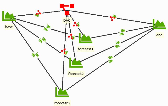
The stochastic_scenario_end parameter starts counting from the start of the simulation! In the examples above, when the base stochastic_scenario has a duration of 6h and the forecast stochastic_scenarios have a duration of 16h, the forecast stochastic_scenarios will only be active for 10 hours between hour 6 and hour 16!